The Randles Circuit
The Randles circuit is the probably the most recognisable equivalent circuit model in the world of electrochemistry and electrochemical impedance spectroscopy. We’ll look at what processes it models, why the model is arranged in the way it is, and its distinctive Nyquist plot.
The Randles circuit, given below, is a model for a semi-infinite diffusion-controlled faradaic reaction to a planar electrode.

That’s a lot of technical terms, I know. But the Randles circuit has plenty of significance to real electrochemical reactions, and if you’ve already worked your way through the previous pages in this section you should now be familiar with all of the elements.
A simple model for an electrode immersed in an electrolyte is simply the series combination of the ionic resistance, Ri, with the double layer capacitance, Cdl. If a faradaic reaction is taking place, of the sort:
$$\text{O} + \text{e}^- \rightleftharpoons \text{R} $$then that reaction is occurring in parallel with the charging of the double layer – so the charge transfer resistance, Rct, associated with the faradaic reaction is in parallel with Cdl.
The key assumption is that the rate of the faradaic reaction is controlled by diffusion of the reactants to the electrode surface. The diffusional resistance element (the Warburg impedance, W), is therefore in series with Rct.
And that’s all there is to it. You will see impedance responses with this sort of shape in all manner of electrochemical systems, although often with multiple semicircles and other overlapping processes.
Nyquist and Bode plots
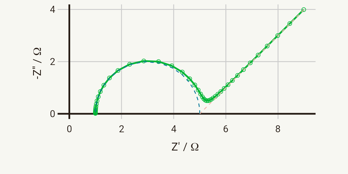
A typical Nyquist plot for the response of a Randles circuit is shown below. The distinctive shape of the Nyquist plot for the Randles circuit is the semicircle created by the Ri-(RctCdl) portion of the circuit, followed by the 45° line characteristic of the Warburg impedance. These two separate parts of the circuit are indicated by the dotted lines on the plot.
The Bode plot for the same circuit follows below. As you will have seen on previous pages, we can similarly extract the relaxation frequency for the RctCdl time constant from the peak in Z’’ in the Bode plot.
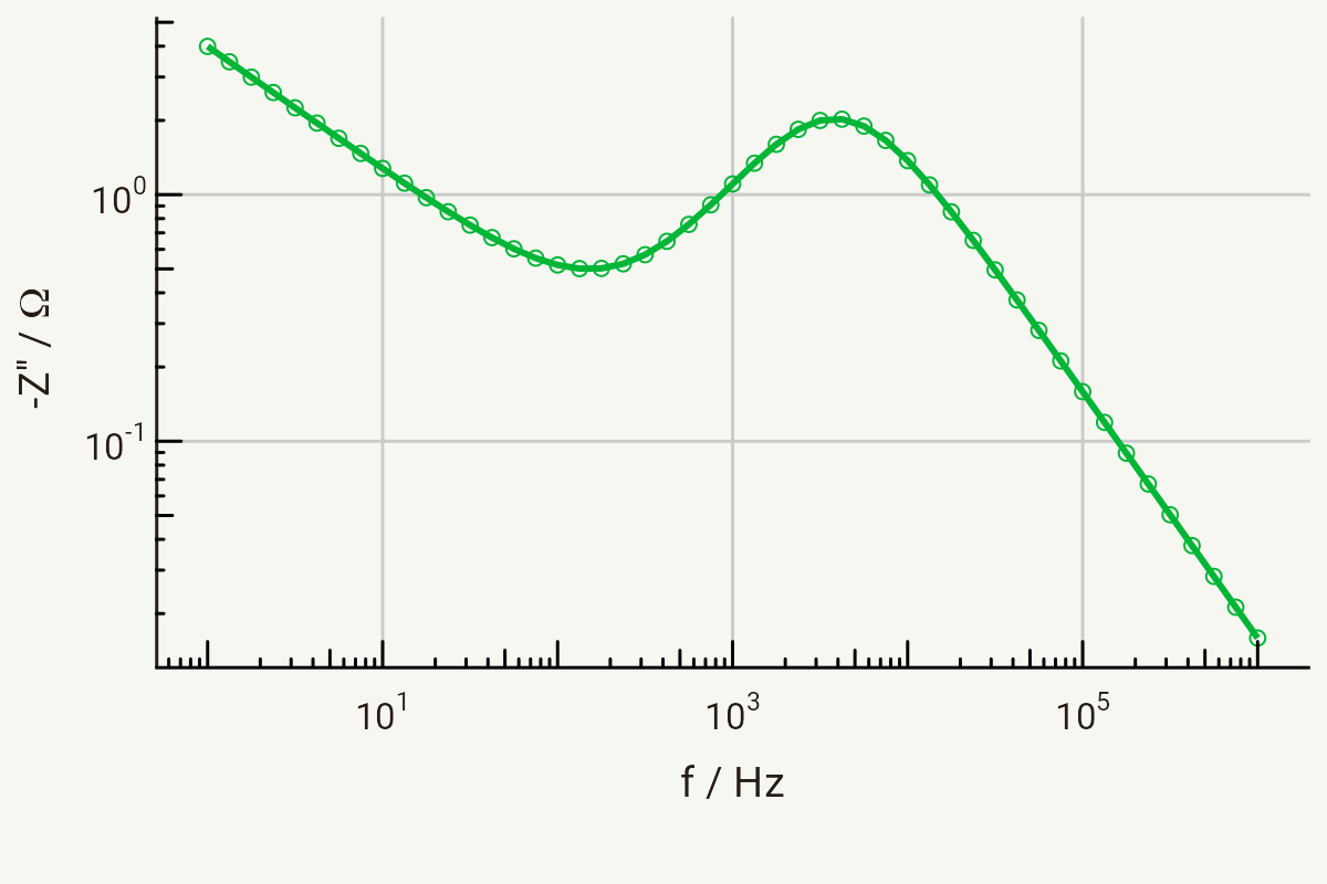
Parameters for both of these plots: Ri = 1 Ω, Rct = 4 Ω, Cdl = 10-5 F, σ = 10 Ω s-1/2, in the range 1 MHz - 1 Hz.
A note on series and parallel combinations
The question of whether elements corresponding to physical processes should be in series or in parallel in a circuit model can often cause confusion. An important aspect to consider is whether the current which is associated with each element either adds to the currents from other processes, or limits (or is limited) by them.
In the case of the Randles circuit, the faradaic current (which flows through the Rct resistor) and the capacitive current (which flows through the Cdl element) are independent of each other, and as a result are additive:
$$I_\text{total} = I_\text{faradaic} + I_\text{capacitive} $$The currents flowing in circuit elements which are in parallel add together to give the total current in the circuit, so physical processes which independently contribute to the total current are typically represented in parallel.
Conversely, if two processes act as a bottleneck for each other, the same current flows through both elements and they are therefore usually represented in series. In series, as we have seen earlier, the impedances of each element are additive.