Fitting With Real Data

I know from personal experience that knowing the basics well enough to interpret a very simple and well-defined experiment is one thing – but actually taking that knowledge and trying to make sense of the response of a complex ‘real’ system is another.

As equivalent circuits become more complicated, they become harder to fit correctly. Impedance software uses non-linear least squares regression to fit the data to the models, and they need reasonable values to start with to converge on a solution. The more complicated the model gets, the more likely the software is to fail in its attempt to fit the data – or it returns a fit which looks ok on the plot but has huge errors for some of the terms.

It’s this aspect of practical EIS which I think makes it hard to learn, and I don’t think there’s a lot of help out there for users who don’t have the luxury of being able to consult a local expert.

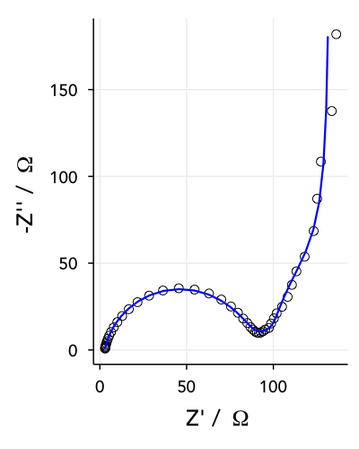
On the previous page, on three- and four-electrode measurements, I showed some real data from a Li-ion test battery just after assembly, and a rather complicated suggested equivalent circuit for it. You might have also recognised that the Nyquist plot for the positive electrode (taken from a 3-electrode measurement) was the same as I showed on the main page of this guide (shown again on the right) – and maybe you’re wondering where the equivalent circuit came from.

Well, the equivalent circuit I’ve chosen is somewhat empirical – and I’m not going to guarantee that it’s the most appropriate possible circuit – but I figured it makes a convenient example to show you how you can approach fitting a more complex dataset. On this page I’ll detail the process I used to analyse the data by eye and build up the model.

Equivalent circuit fitting in ZView

The screenshots I present here are from ZView, which can be downloaded from the software manufacturer, although the latest versions will only run in ‘demonstration mode’ – which is basically unusable – unless you have an expensive licence. Older versions (e.g. 3.2b) are ok, and Google may help you find it…

Ok, to the data. Let’s look at the spectrum above again, and pretend the fit line isn’t there. What are the obvious features? Well, there’s the slightly depressed semicircle at high frequency, and then the behaviour is pseudocapacitive at lower frequencies (lowest frequency is 100 mHz, incidentally).

Essentially, the strategy I use is quite simple: fit the obvious stuff first, and then build up the rest of the model around that. Have a look at the following screenshot (you can click on it to enlarge it):

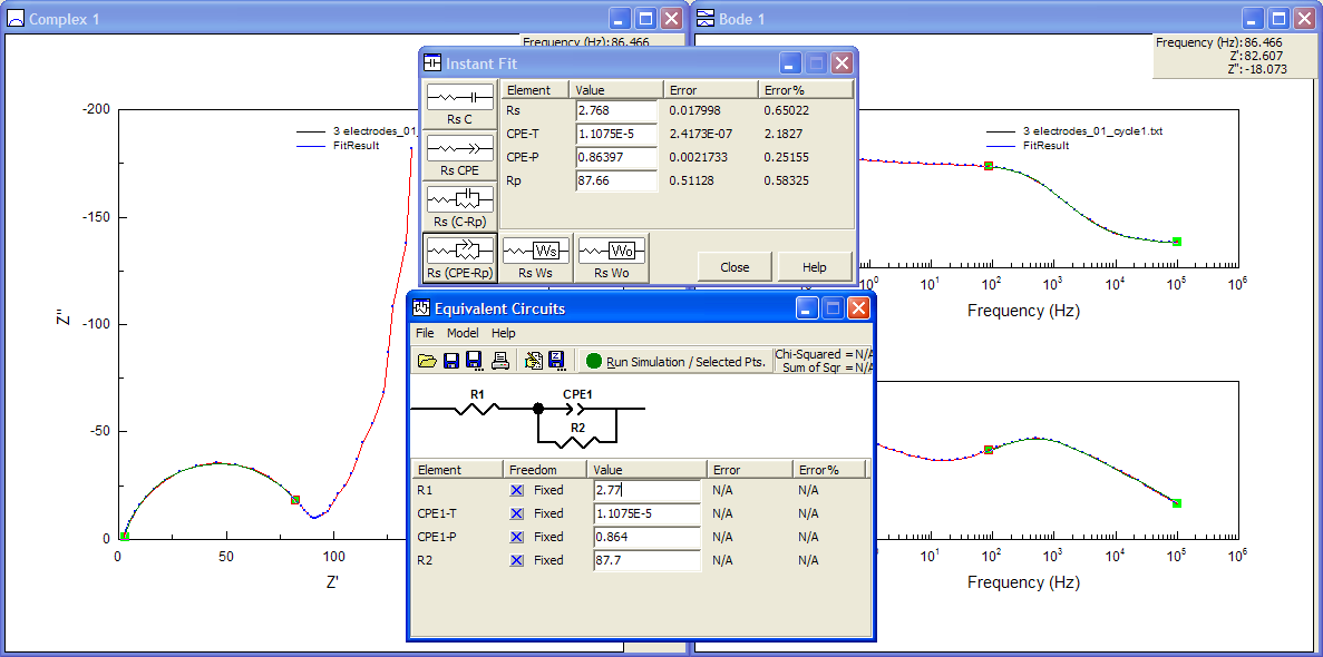
ZView lets you use sliders to fit only a part of the data if you want, and this is invaluable. Also very useful is ZView’s “Instant Fit” tool, which will fit the selected data only to any of six very simple equivalent circuits, without needing any starting values from the user. So a good place to start here, especially if you have no idea what values might be appropriate, is to fit the semicircle with the Rs (CPE-Rp) circuit (bottom-right in the Instant Fit window). As you can see, the fit is pretty good, with small errors, so I’ll take the numbers from the Instant Fit and start building up my own model in “Equivalent Circuits”.

Now to fit the low-frequency tail. I could try to fit it with a constant phase element, but the phase is obviously changing, so it’s probably not appropriate. I can try to fit it anyway just to show that it doesn’t fit well, even though the errors come out to be rather small:

The advice I often give to people who ask me about EIS measurements is that it helps to know what the spectrum should look like, although that isn’t always possible. At this point I should probably make a guess based on what I’m actually measuring. Since the electrode is for the most part a Li-ion battery positive electrode, there’s Li ions in the material which are probably moving around in response to my applied potential. So I can try to put a finite space Warburg (or “open” Warburg, in ZView language) to model that finite diffusion behaviour, instead of that CPE I tried earlier.

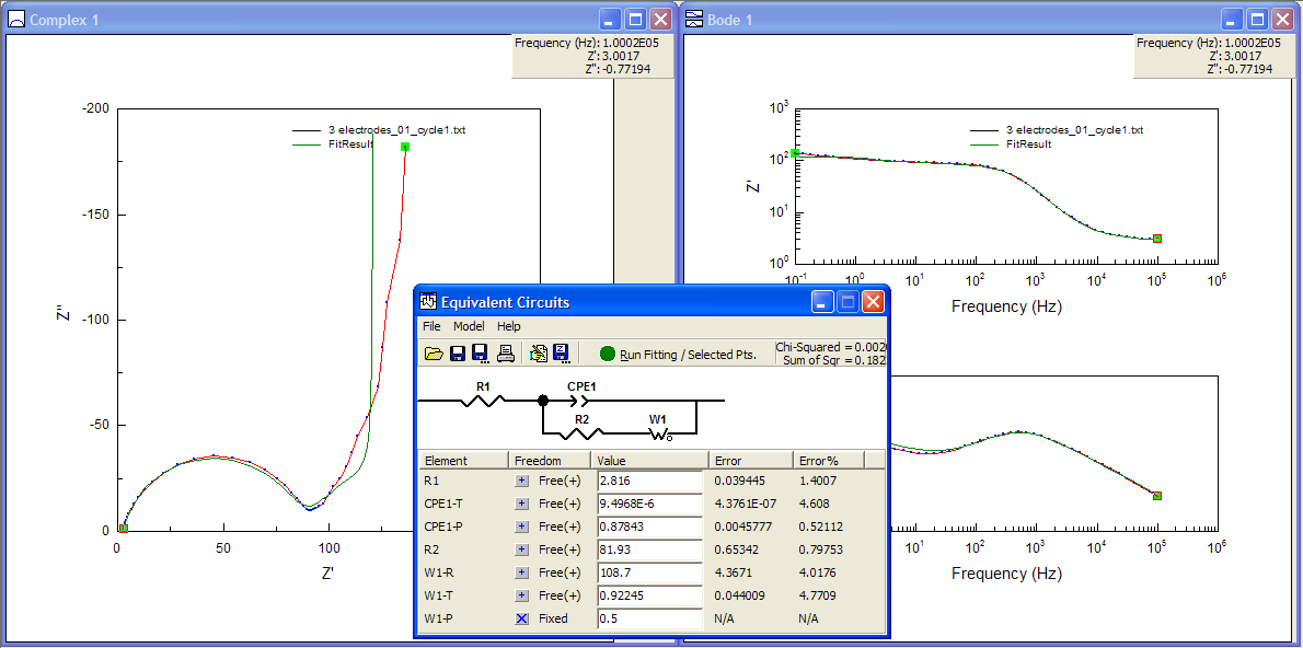
Well, it’s not really much better, though it makes a bit more sense… and it does fit that very first bit of the Nyquist plot after the semi-circle a bit better (the very short 45° part where Z’ ~ 90 Ω), so maybe I’m onto something.

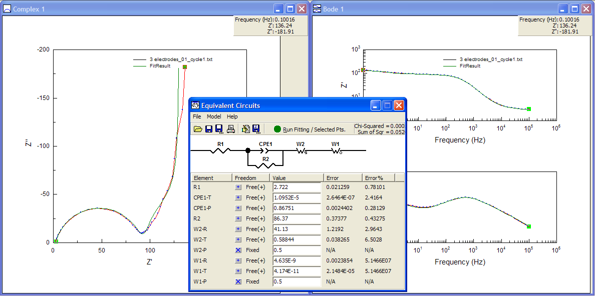
I also know that the electrode is porous, and that porosity can be represented by a finite length Warburg (or “short” Warburg, in ZView terms). So I can try to include this in the model, also in series with the FSW and the resistor R2. I fixed terms initially so that the software only guessed values for the -R (resistance) and -T (time constant) terms for the new FLW element (using 1 for each of the terms as a starting point), and then re-ran the fitting with other values freed up, keeping the phase of the Warburgs at 45° (P = 0.5).

So, now the fit is fairly decent – although the errors of 12% for the FSW element give me a little cause for concern. I could un-fix the phase angles as well – and I did, and the fit to the Nyquist plot looked better – but it caused some of the errors associated with the elements to hit more than 500%! In that case, you really can’t be sure the model is a good one.

Perhaps I can try something else. What if I try again with the Warburg elements in series with the CPE instead of in parallel with it?

Well, the fit in the Nyquist plot looks ok, similar to the last one, maybe except for that first bit of the tail… oh, wait. The values for the FSW (W1-T and W1-R) have become absurdly small and the errors are 50 million percent! That’s a telltale sign of having screwed up.

Wrap-up

Well, I concede I probably haven’t reached anything conclusive here, but if you’re new to EIS you now hopefully have at least a bit of an idea of how you can approach an equivalent circuit fitting, and some appreciation for some of the difficulties.

It’s an anticlimax, I suppose, but I do have a reason. When I was a lab teacher for EIS at the Southampton Electrochemistry Summer School, we ran a few very well-designed experiments which we knew would give easy-to-understand results; the most in-depth experiment was an analysis of the ferricyanide redox couple at a mirror-smooth glassy carbon electrode, where you get a very lovely Randles circuit response and it’s dead easy to fit and extract a load of meaningful parameters from. This is great for learning about the technique, but of course the delegates – mostly not academics – ultimately wanted to know how to apply it practically to their own work. We often got questions about predicting or analysing impedance spectra of much more complex systems like these, and we weren’t always able to give a clear answer.

The truth is that real-world EIS is more like this example here, in my experience. The more you want to learn the more you have to think about the design of the experiment, sometimes you have to take an educated guess at an appropriate equivalent circuit, and even then it can be difficult to be sure. Hence this example – it was genuinely my first attempt at fitting this data, so this was my real thought process.

Perhaps I’ve ended this example pessimistically. I don’t mean to – EIS is still a very useful technique. It’s fast, you get a lot of information that few other techniques can give you as easily – but sometimes you’ve got to be realistic about how much quantitative analysis you can do with it, and careful that when you do that analysis, the model and numbers make sense.

Get involved