Multiple Time Constants
Here, we’ll look at the series combination of two parallel RC circuits, and in particular how the relaxation time constants influence our interpretation of the results.
Let’s consider the impedance of this circuit:

If you have familiarised yourself with the contents of the previous page you should recognise that we can calculate the impedance of this circuit, which we can refer to as an RC-RC circuit, by this equation:
$$\pmb{Z} = \frac{R_1}{1 + j \omega R_1 C_1} + \frac{R_2}{1 + j \omega R_2 C_2} \tag{1}$$You might also see from this equation that we expect the response of this RC-RC to be two semicircles, one for each separate parallel RC ‘unit’, each with their own RC time constants. But how do we know which semicircle corresponds to which parallel RC ‘unit’?
The critical thing to understand is that, in a Nyquist plot, the semicircles appear in order of increasing time constant (and, in turn, decreasing relaxation frequency). Parallel RCs with a smaller RC time constant (smaller $R \times C$ product) will appear first, at higher frequencies, and higher time constant processes will appear later, at lower frequencies.
To illustrate this, we can consider the response of a hypothetical circuit as illustrated above, with fixed resistors but capacitors of different values, to vary the RC time constants. In the below example, we have R1 = 5 Ω and R2 = 15 Ω, and the following three cases where τ1 = R1C1 and τ2 = R2C2:
- C1 = 10-5 F, C2 = 10-3 F; therefore τ1 < τ2
- C1 = 10-3 F, C2 = 10-5 F; therefore τ1 > τ2
- C1 = 10-4 F, C2 = 3.3 × 10⁻³ F; therefore τ1 = τ2
The Nyquist plots of these cases is given below:
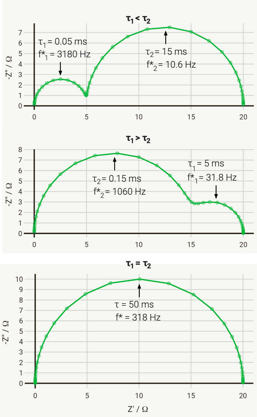
As you can see, in the first case the 5 Ω semicircle appears on the left of the Nyquist due to its lower time constant. In the second case, swapping the parallel connected capacitors over changes the time constant, so that the 5 Ω semicircle has a larger time constant, has therefore a lower relaxation frequency, and instead appears on the right of the Nyquist plot.
In the third case, the capacitances have been selected so that the time constants are equal. In this case, the two capacitors charge at exactly the same rate, and the response of the circuit will be identical to that of a single parallel RC circuit, with a total resistance at zero frequency (DC) of R1 + R2.
This last case has significant practical implications, as it tells us that if we have two separate processes with very different associated R and C values, if they have similar or equal time constants (i.e., they occur on a similar time scale), then they may be extremely difficult (or impossible) to separate. This is a fundamental challenge with EIS.
We can also visualise this with the below animated plot (kindly provided by Dr Sam Cooper). The below plot similarly shows an R-RC-RC circuit where one capacitor value is varied (all other components fixed) to change the time constant, and the order in which they appear. You will see that the closer the two time constants are to each other, the more they overlap.