This introduction to electrochemical impedance spectroscopy (EIS) began in 2016 as a result of what I saw as a lack of easily accessible and useful information for learning the principles, theory and practical application of EIS for most users (that is, non-electrochemists). The way I saw it, there was very little help available for those who got the basic idea of EIS but were struggling to fit their data or weren’t sure how to set up their experiments. If you’re looking to get a handle on EIS but aren’t sure where to start, these pages are, hopefully, for you.
The pages that follow include basic explanations starting from the beginning, along with some simulation web apps and some exercises where you can get a feel for working with impedance data. You can get started by following the links below, or in the main menu. Comments and suggestions for the Content Roadmap are always very welcome.
First off, I want to say that although I’ve been a user of impedance spectroscopy since 2008, on an applied level (battery characterisation) it still confuses the hell out of me on a regular basis. Learning the theory is one thing, but in-depth analysis, especially when it comes to equivalent circuit fitting, is hard – it requires a healthy degree of intuition, and usually needs very carefully designed experiments to get meaningful results… but sometimes it’s just a pain. I’d dare to suggest that a large proportion - maybe even a majority - of the people in the battery field who have done some impedance spectroscopy work in peer-reviewed publications do not really understand what they’re doing with it.
But, don’t be discouraged(!). It’s not easy to learn, but in writing this I’ve done my best to keep the level as accessible as possible, to give examples, some little apps where you can do simulations to see how changing parameters in a model system changes things, and many more, to try and give you the best chance to build up that level of intuition.
I used to finish my lectures with “Matt’s top tips for impedance spectroscopy”, to try to restore some of the enthusiasm and confidence I’ve just stolen from my poor students, and here they are:
Matt’s top tips for impedance spectroscopy
EIS can be ambiguous, and a good equivalent circuit fit can be elusive (but don’t let that put you off)
The fewer parameters an equivalent circuit has, the better
Always check the fitted values make sense (and the errors are reasonable).
Practice makes perfect!
Download [some simulation/fitting software of your choice] and play around*…
* An example is ZView (Scribner Associates). Older versions (e.g. 3.2) allow you to do simulations as well as equivalent circuit fitting of data. Perhaps Google can help you out…
Get involved
Subsections of Electrochemical Impedance Spectroscopy (EIS)
Principles of EIS
1231 words (6 min) Matthew Lacey 15 Feb 2023
Defence against the dark arts
Since you’re reading this, you most likely know that as the name suggests, Electrochemical Impedance Spectroscopy (or just EIS, from now on) involves looking at the impedance characteristics of an electrochemical system over a range of frequencies (that’ll be the spectrum part). And maybe you’re thinking about trying your hand at some equivalent circuit fitting, which is the dark art process of fitting a spectrum you’ve measured to a model based on some real (and some not real) electrical components. But first, it’s important to understand some of the theory behind impedance itself.
Impedance vs resistance
Consider Ohm’s law, which describes the relationship of voltage to a direct current passing through a resistor:
$$E = IR \tag{1}$$
Impedance is, very simply, extends the concept of resistance to an alternating current, and generally represented as
$\pmb{Z}$. So you can think of it, simply, like this:
$$E = I\pmb{Z} \tag{2}$$
We’ll come back to this in a moment. For now, it should be clear that a measurement of impedance, therefore, can be made by made simply by applying an oscillating voltage, and measuring the (oscillating) current response. We can write down an equation for the oscillating voltage we apply like so:
$$E(t) = \left|E\right|\sin(\omega t) \tag{3}$$
where
$\left|E\right|$ is the amplitude of the voltage signal, and
$\omega = 2 \pi f$ (the angular frequency). The response will be a current with an amplitude
$\left|I\right|$, which is also shifted in phase from the applied signal:
$$I(t) = \left|I\right|\sin(\omega t + \theta) \tag{4}$$
The current is shifted in phase because of reactance (e.g., a capacitance or inductance) in addition to the resistance (which changes the amplitude). The impedance can therefore be expressed like this:
$$\pmb{Z} = \frac{E(t)}{I(t)} = \frac{|E| \sin(\omega t)}{|I| \sin(\omega t + \theta)} = |Z| \frac{\sin(\omega t)}{\sin(\omega t + \theta)} \tag{5}$$
Have a look at the animation below. The ‘current’, I, is 72° out of phase with the ‘voltage’. The graph on the right is known as a Lissajous curve, showing the relationship between I and E. In the past, impedance spectroscopy was done by obtaining these curves on an oscilloscope and analysing them. Thankfully, it’s all a bit easier nowadays.
Impedance as a complex number
Ok, complex maths time. Without going into too much detail, via Euler’s formula:
$$e^{jx} = \cos(x) + j \sin(x) \tag{6}$$
we can re-write all of the above using complex numbers:
$$\pmb{E} = I \pmb{Z} = I\left|Z\right|e^{j \theta} \tag{8}$$
Note that
$j$ is the imaginary unit, i.e.,
$j = \sqrt{-1}$, which we use instead of
$i$ to avoid confusion with the symbol for electrical current. You can see from the above equation that the ratio of an oscillating voltage to an oscillating current is the impedance, which has a magnitude
$|Z|$ and a phase angle
$\theta$. You can think of this as a polar coordinate representation. More commonly for impedance spectroscopy, however, we generally use the Cartesian complex plane representation, dividing the complex impedance into the real and imaginary parts:
$$\pmb{Z} = Z' + j Z'' \tag{9}$$
$Z'$ and
$Z''$ are the resistive and reactive parts of the impedance respectively. You’ll see this more clearly on the page about the impedance of simple RC circuits.
We can represent any
$\pmb{Z}$ on an Argand diagram, as in the graph below. This is the basis for the Nyquist plot, which is the plot of the real and imaginary parts of the impedance that you’ll come across most often. An impedance measurement for a single frequency is a single point on a Nyquist plot. An impedance spectrum is therefore a series of points, where each point is a different frequency.
These plots are visually useful, because the characteristic shapes that can appear in the plots as you’ll see later can give you a rough idea of what you’re looking at. The downside, though, is that you can’t know what the frequency associated with a particular point is from looking at the Nyquist plot alone, and so the plot doesn’t contain all the information you need. This is why the alternative Bode plot – plots of
$\log Z'$ and
$\log Z''$ vs
$\log f$, or
$\log |Z|$ and
$\theta$ vs
$\log f$ – are still important.
Nyquist plot
I’ll finish up this page by briefly introducing a typical Nyquist representation of an impedance spectrum itself. The plot below is data I acquired from a Li-ion test battery, and fitted to a model myself. The frequency range the points represents is between 100 kHz and 100 mHz. This is fairly typical for most systems, although depending on what you want to measure you might go up to 1 MHz or more, or as low as 1 mHz. So how do you make sense of this plot? Well, there are three things I’ll note for now.
First, the impedance is always lowest (i.e., smallest values of
$|Z|$ at the highest frequency, so you can see that the frequency decreases if we follow the curve from the points near the origin to the points in the top-right corner. Secondly, you’ll note (as in the Argand diagram above) that the values of
$Z''$ are negative (plotted as
$-Z''$). This will become clearer later, but by convention capacitance is a negative reactance, so impedance spectra will in most cases only have positive
$Z’$ values and negative
$Z''$ values.
Lastly, you’ll note the shape of the spectrum, particularly the semi-circle part. The shapes you see in the Nyquist plots can be characteristic of certain elements or combinations of elements, so they are (often, but not always) visually useful for quickly understanding something about the system you’re measuring. Because of this I was able to take this relatively good quality data, think of a reasonable model, guess a few of the parameters and then fit the entire spectrum relatively quickly. In the following pages you’ll read about the experimental technique I used to get this data as well as the elements of the model I’ve fitted the data to, and hopefully you’ll be able to see how it all fits together.
Square the axes!
There’s a slightly nitpicky but formal stylistic point I like to make when I give lectures on this topic, and that’s about axis scaling on Nyquist plots. As you can see from my Argand diagram above, the axes are proportional (i.e., 2 units on the x-axis are equal in length to 2 units on the y-axis). Formally, it should be this way, because you can still read any point as a magnitude and a phase angle as well as the real and imaginary parts. Practically, it is still helpful to do this because it will let you see important features such as 45° lines easily. Unfortunately, most people who publish impedance results in the literature do not do this. To some extent, I sympathise, because common scientific graphing programs like Origin Pro do not make it easy to do this. But, most often the person making the graph goes to the effort to set the limits on the x- and y-axes to be the same, but keeps the plot itself the default rectangle, rather than resizing it to a square. This, I think, is just sloppy.
And as a final tip for R and ggplot2 users: it is thankfully trivial to ensure that axes are kept proportional. Just add coord_fixed to ggplot()!
Get involved
RC circuits
1161 words (6 min) Matthew Lacey 15 Feb 2023
Overview
Now that we’ve introduced some of the maths behind impedance, and the plots we use to represent it, we can start to look at the mathematical definitions and the impedance response of two of the most basic electrical circuit components – resistors and capacitors – and combinations of them.
Impedance of a resistor
This is the simplest electrical circuit, and the easiest to understand. Resistors, as you surely know, obey Ohm’s law, so the current is always proportional to the voltage, there is no reactive part (i.e., phase shift) and so no dependence on frequency whatsoever. We can just write that down like this:
$$\pmb{Z}_R = R \tag{1}$$
where R is the resistance. The Nyquist plot for a resistor then is very simple – it’s just a single point on the x-axis at any frequency. The below plot shows the Nyquist plot for a resistor with a resistance of 20 Ω.
Impedance of a capacitor
Capacitors have a purely reactive impedance. An ideal capacitor has zero resistance. When an alternating voltage is applied across a capacitor, the current leads the voltage (the phase is -90°), and the impedance is inversely proportional to the frequency. That is, the impedance increases with decreasing frequency. Consider applying a DC voltage across a capacitor – after a long enough time, the capacitor is fully charged and no more current flows. The impedance is effectively infinity. The equation describing a capacitor is:
$$\pmb{Z}_C = \frac{1}{j \omega C} \tag{2}$$
where
$j$ is the imaginary unit,
$\omega = 2 \pi f$ and
$C$ is the capacitance.
he Nyquist plot for a capacitor therefore looks like a vertical line, where Z’ = 0 for all frequencies. The below plot shows the Nyquist plot for a capacitor with a capacitance of 1 mF, in the frequency range 1 kHz – 10 Hz. The highest frequency points have the lowest impedance, with the impedance increasing as frequency decreases.
Capacitances arise all over the place in electrochemical systems, pretty much anywhere you have an interface – most often from the capacitance of the double layer, but also dielectric capacitance, or at grain boundaries in solids, and so on.
This is all fairly straightforward so far, so now we’re going to consider combining some of these different circuits together.
RC circuits
Series RC circuit
In series, the impedances are additive:
$$\pmb{Z} = \sum_n \pmb{Z}_n \tag{3}$$
The impedance of the series RC circuit is therefore just the addition of the individual impedances of the resistor and the capacitor together:
The Nyquist plot for a series RC circuit (where R = 5 Ω, C = 1 mF, in the frequency range 1 kHz – 10 Hz) is shown below. As you might expect, the real impedance Z’ is equal to the resistance of the resistor for all frequencies, and the imaginary part of the impedance follows the same behaviour as for the ideal capacitor.
You can consider the series RC circuit as a simple model for things like a blocking interface – for example an inert electrode immersed in a conducting electrolyte – where R represents the ionic resistance of the electrolyte, and C represents the capacitance of the double layer on the electrode surface.
This also represents two electrodes in an electrolyte (i.e., a complete cell), because a series circuit with two capacitors (i.e., C-R-C) simplifies down to a single RC unit anyway, if you follow the equations above.
Parallel RC circuit
Now, let’s consider the parallel case.
In parallel, the admittances (i.e., the reciprocals of the impedances) are additive:
So then we can write the expression for the parallel RC circuit like so:
$$\frac{1}{\pmb{Z}} = \frac{1}{R} + j \omega C \tag{6}$$
If we rearrange that equation for
$\pmb{Z}$ (by first multiplying all the terms by R) then we end up with:
$$\pmb{Z} = \frac{R}{1 + j \omega RC} \tag{7}$$
From this equation you can see that at high frequency, i.e.,
$\omega \rightarrow \infty$, the lower term on the fraction goes to infinity, so the impedance tends towards zero; the ideal circuit behaves like the capacitor at infinite frequency – it has zero impedance. At low frequency, i.e.,
$\omega \rightarrow 0$, however, you can see that the bottom term becomes 1, so the total impedance of the circuit equals R – i.e., with a direct current, the circuit behaves like a resistor (this makes sense, right? Eventually with a direct current, the capacitor becomes fully charged and the current only goes through the resistor). The Nyquist plot for this circuit, then, is a semicircle, intercepting the real (Z’) axis at 0 and R. The below plot shows the Nyquist plot for a parallel RC circuit where R = 5 Ω, C = 1 mF, in the frequency range 1 kHz – 1 Hz:
Semicircles in the Nyquist plot are very common in electrochemical impedance, and are usually associated with processes such as charge transfer, because at an electrode surface the transfer of charge happens in parallel with the charging of the double layer capacitance – hence the semicircle.
You’ll also note that I’ve marked the very top of the semicircle with f*. This is known as the relaxation frequency, and relates to the RC time constant of the circuit. From the previous equation, you will see that the peak of the semicircle occurs when
$\omega RC = 1$. The time constant is then defined as follows:
This is an important concept in EIS, because it tells us something about the timescales on which different processes are occurring. This equation also allows you to calculate capacitances in these elements knowing only the resistance (from the diameter) and the relaxation frequency.
This is where the Bode plot comes in handy. The top of the semicircle simply appears as a peak in a plot of the imaginary part against the frequency, with log scaling:
Since I simulated the circuit with values of R = 5 Ω and C = 1 mF, you should be able to follow that:
and see on the Bode plot above that the peak is at around 32 Hz.
Another reason this is important is that the time constant (that is, the frequency dependence) of these elements of course affects the order in which they appear in the Nyquist plot. Elements with a smaller time constant (i.e., a higher relaxation frequency) will, naturally, appear at higher frequencies in the impedance spectrum. Of greater concern, however, is that elements with very similar or the same time constants will tend to overlap. I’ve included a Shiny app for simulating a circuit made up of two parallel RC units in series to show this. Have a go at changing the parameters, and see how they affect what the Nyquist plot looks like.
Get involved
Multiple Time Constants
537 words (3 min) Matthew Lacey 28 Mar 2023
Overview
Here, we’ll look at the series combination of two parallel RC circuits, and in particular how the relaxation time constants influence our interpretation of the results.
Let’s consider the impedance of this circuit:
If you have familiarised yourself with the contents of the previous page you should recognise that we can calculate the impedance of this circuit, which we can refer to as an RC-RC circuit, by this equation:
You might also see from this equation that we expect the response of this RC-RC to be two semicircles, one for each separate parallel RC ‘unit’, each with their own RC time constants. But how do we know which semicircle corresponds to which parallel RC ‘unit’?
The critical thing to understand is that, in a Nyquist plot, the semicircles appear in order of increasing time constant (and, in turn, decreasing relaxation frequency). Parallel RCs with a smaller RC time constant (smaller
$R \times C$ product) will appear first, at higher frequencies, and higher time constant processes will appear later, at lower frequencies.
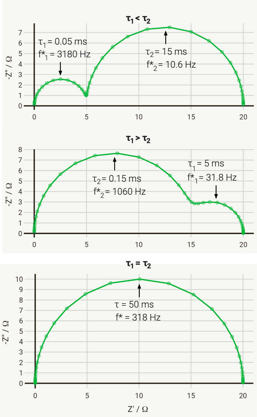
To illustrate this, we can consider the response of a hypothetical circuit as illustrated above, with fixed resistors but capacitors of different values, to vary the RC time constants. In the below example, we have R1 = 5 Ω and R2 = 15 Ω, and the following three cases where τ1 = R1C1 and τ2 = R2C2:
C1 = 10-5 F, C2 = 10-3 F; therefore τ1 < τ2
C1 = 10-3 F, C2 = 10-5 F; therefore τ1 > τ2
C1 = 10-4 F, C2 = 3.3 × 10⁻³ F; therefore τ1 = τ2
The Nyquist plots of these cases is given below:
As you can see, in the first case the 5 Ω semicircle appears on the left of the Nyquist due to its lower time constant. In the second case, swapping the parallel connected capacitors over changes the time constant, so that the 5 Ω semicircle has a larger time constant, has therefore a lower relaxation frequency, and instead appears on the right of the Nyquist plot.
In the third case, the capacitances have been selected so that the time constants are equal. In this case, the two capacitors charge at exactly the same rate, and the response of the circuit will be identical to that of a single parallel RC circuit, with a total resistance at zero frequency (DC) of R1 + R2.
This last case has significant practical implications, as it tells us that if we have two separate processes with very different associated R and C values, if they have similar or equal time constants (i.e., they occur on a similar time scale), then they may be extremely difficult (or impossible) to separate. This is a fundamental challenge with EIS.
We can also visualise this with the below animated plot (kindly provided by Dr Sam Cooper). The below plot similarly shows an R-RC-RC circuit where one capacitor value is varied (all other components fixed) to change the time constant, and the order in which they appear. You will see that the closer the two time constants are to each other, the more they overlap.
Get involved
Constant Phase Elements
601 words (3 min) Matthew Lacey 28 Mar 2023
Overview
So far, we’ve looked at the impedance response for some ideal resistors and capacitors and some simple combinations of them. Unfortunately, in electrochemical systems we often encounter processes which don’t have a “real” equivalent electrical component, so we have to invent some. One of the most common such elements is the constant phase element, or CPE.
One of the most common circuit elements for modelling non-ideal behaviour is the constant phase element (CPE, or sometimes Q). This is a common symbol for this circuit element:
You might think that it looks like a wonky capacitor – and you’d be right, because this circuit element exists largely to describe capacitance as it appears in real electrochemical systems, because of things like rough surfaces, or a distribution of reaction rates. It is an imperfect capacitance – the effective capacitance and ‘real’ resistance are increasing as the frequency decreases. The origins of CPE behaviour are numerous and some of them quite complex, but there are good guides explaining this elsewhere.
The mathematical definition is very similar to that of the capacitor as well:
$$\pmb{Z}_Q = \frac{1}{Q_0 (j \omega)^n}$$
where n is the constant phase,
$(-90 \times n)$°, and n is a number between 0 and 1. Be aware though – this is not the only possible definition of the constant phase element – it can also be defined by putting the Q0 value inside the brackets.
So, what does the Nyquist plot look like? You might have guessed by now that the Nyquist plot for a CPE looks similar to a capacitor – a straight line, but with a phase of
$(-90 \times n)$°. The below plot shows the Nyquist plot for a CPE with a Q of 1 mS sn, where n = 0.85 (more on those units later), in the frequency range 1 kHz - 10 Hz.
R-CPE or RQ circuits
It should be fairly clear by now what the Nyquist plot of a series R-CPE element looks like, so I’ll only show the parallel case, the characteristic “depressed” semicircle. The below plot shows the Nyquist plot for a CPE with a Q of 1 mS sn, where n = 0.85, in parallel with a 5 Ω resistor, in the frequency range 10 kHz - 10 Hz.
The Bode plot for a parallel R-CPE circuit looks very similar to that of a parallel RC circuit, but with a subtle difference: on a log-log plot (i.e., log(-Z’’) vs log f), the gradient of the straight line gives you the n value:
You may be able to see from the above plot that in the high frequency region (to the right of the peak) the gradient is -0.85, and in the low frequency region (to the left of the peak) the gradient is +0.85. Being able to estimate these values from Bode plots can be a useful technique to estimate parameters when performing equivalent circuit fitting, as we will see later on in this section.
Can I calculate the real capacitance?
Q0, according to the mathematical definition of the CPE, has units of S sn (that’s siemens-seconds-to-the-power-n), which have no real physical meaning. However, it is possible to determine the actual capacitance behind the CPE when you have a parallel R-CPE circuit. Think about the units again – you should be able to see that:
$$RQ_0 = \tau^n = (RC)^n$$
Rearranging this equation gives:
$$C = \frac{(RQ)^{\frac{1}{n}}}{R}$$
This equation holds as long as the phase angle does not deviate too far from -90° (n > 0.75). I won’t go into this further, though – the ConsultRSR webpages on EIS provide some useful reading on this point.
Get involved
Diffusion Impedance
1131 words (6 min) Matthew Lacey 28 Mar 2023
Overview
Mass transport processes, such as diffusion, migration and convection, are a key aspect of electrochemical systems. In this subsection, we will look at fundamental models for the effect of diffusion processes on impedance. As with the CPE, we invent some new circuit elements to describe these, but these can be approximated using the familiar resistors and capacitors, as we will see.
Semi-infinite diffusion
The simplest and most common circuit element for modelling diffusion behaviour is the Warburg impedance or Warburg element, which models semi-infinite linear diffusion – that is, diffusion in one dimension which is only bounded by a large planar electrode on one side.
The equation for this element is relatively simple:
where
$\sigma$ is the Warburg coefficient, with units of Ω s-1/2 – we’ll come back to this shortly. In the Nyquist plot, the Warburg impedance gives a straight line with a phase of 45°, which is very recognisable in EIS. If you spot a 45° line in the Nyquist plot, it is usually associated with diffusion. The below plot shows the Nyquist plot for a Warburg element with
$\sigma$ of 10 Ω s-1/2 in the frequency range 10 kHz - 10 Hz.
And if you’re looking at this thinking that this line look very much like a constant phase element but with a phase angle of 45°, then you’d be right – mathematically they are very much the same. In fact, some popular impedance analysis softwares do not actually provide a semi-infinite Warburg element, so a convenient alternative for this is a CPE element with n fixed at 0.5. This gives slightly different numbers back when fitting – if you use a CPE, you will get back the Q0 value, rather than the Warburg coefficient
$\sigma$. The two values are related though, by the equation:
$$\sigma = \frac{1}{\sqrt{2} \cdot Q_0} $$
But what does
$\sigma$ actually mean? This is somewhat more complicated, but if you consider the case where you have a soluble redox couple in solution, with a nice reversible electrochemical reaction like:
$$\text{O + n e}^- \rightleftharpoons \text{ R} $$
then
$\sigma$ is related to the diffusion coefficients and concentrations of those species:
here, in addition to the usual constants,
$D_O$ and
$D_R$ are the diffusion coefficients and
$c^\infty_O$ and
$c^\infty_R$ are the bulk concentrations for the species O and R respectively.
The transmission line
Conventional “Fickian” diffusion is not the only process which gives rise to this type of impedance in electrochemical systems. In batteries, the porosity of electrodes also gives rise to a similarly characteristic 45° line in the Nyquist plot.
This was described in detail by de Levie, who proposed the transmission line model for an electrode with cylindrical pores filled with electrolyte:
Consider the two parallel “rails” as being the electronic resistance in the electrode material itself and the ionic resistance in the electrolyte respectively. The capacitors represent the double layer capacitance.
This equivalent circuit, when infinitely long, gives an impedance response which is identical to the Warburg impedance above. Practically, however, porous electrodes have a finite length, and so show a 45° line only in a certain frequency range. The impedance response due to finite diffusion is discussed below.
A final point on the transmission line: if the transmission line shows the same response as Fickian diffusion, can the case of a porous electrode be considered diffusion as well? In a sense, yes. The movement of ions through the pores is coupled to the movement of electrons through the pore walls. This is an example of ambipolar diffusion.
Finite diffusion
Often in the “classic” electrochemical setups, diffusion often appears semi-infinite because the timescale of the experiment is not long enough for the system to reach a steady state. However, in many real systems and in some standard experiments, diffusion is either naturally, or by design, limited. This gives rise to finite diffusion behaviour, which shows a different response than the standard Warburg impedance.
There are two important equivalent circuit elements for finite diffusion. They are the finite length Warburg (FLW) and the finite space Warburg (FSW), sometimes called the “short” and “open” Warburg elements respectively. Their responses in a Nyquist plot look like this, with parameters Z0 = 10 Ω and
$\tau$ = 0.075 s (more on these parameters shortly) in the frequency range 10 kHz to 10 Hz:
Let’s look at the FLW first. Mathematically, it can be written as:
The two parameters
$Z_0$ and
$\tau$ reflect the properties of the system or the process giving rise to the FLW behaviour. The impedance of the FLW tends to the value of
$Z_0$ at low frequency. At high frequencies, the response is almost exactly that of the Warburg impedance. The shape of the FLW in the Nyquist plot therefore looks like a 45° line at higher frequencies, and transitions into a semi-circle shape at low frequencies. It can be thought of as a Warburg being “shorted” by a resistor - although a parallel W-R circuit will not give the same response. It can also be modelled by a finite length transmission line which is short-circuited at one end. For this reason it is sometimes also known as a “short Warburg”.
This response is typically associated with diffusion (or more generally mass transport) through a layer with a finite length. A classic example of this is the response of the rotating disk electrode - the point of which being to reduce the distance from the electrode to the bulk by controlling convection, rather than diffusion in this case.
In this case, the response tends towards capacitive-like behaviour at low frequencies, where
$Z’(\omega = \infty) = Z_0/3$. This response is typically associated with diffusion where one of the boundaries is blocking, such as in a porous electrode, as discussed previously on this page. This response is also associated with the diffusion of ions within a storage electrode, such as in lithium-ion batteries. This element can also be modelled as a finite length transmission line which is “open” at one end, and for this reason is sometimes also known as an “open Warburg”.
Mind the definitions!
You can find a number of different definitions of these finite elements and it’s easy to get confused. One source of confusion can be from defining these elements in terms of admittance. For example, the FLW is frequently defined like this:
You might have noticed that this definition contains
$\coth$ instead of
$\tanh$. In this case it’s important to remember that:
$$\coth(x) = \frac{1}{\tanh(x)}$$
Get involved
The Randles Circuit
559 words (3 min) Matthew Lacey 28 Mar 2023
Overview
The Randles circuit is the probably the most recognisable equivalent circuit model in the world of electrochemistry and electrochemical impedance spectroscopy. We’ll look at what processes it models, why the model is arranged in the way it is, and its distinctive Nyquist plot.
The Randles circuit, given below, is a model for a semi-infinite diffusion-controlled faradaic reaction to a planar electrode.
That’s a lot of technical terms, I know. But the Randles circuit has plenty of significance to real electrochemical reactions, and if you’ve already worked your way through the previous pages in this section you should now be familiar with all of the elements.
A simple model for an electrode immersed in an electrolyte is simply the series combination of the ionic resistance, Ri, with the double layer capacitance, Cdl. If a faradaic reaction is taking place, of the sort:
then that reaction is occurring in parallel with the charging of the double layer – so the charge transfer resistance, Rct, associated with the faradaic reaction is in parallel with Cdl.
The key assumption is that the rate of the faradaic reaction is controlled by diffusion of the reactants to the electrode surface. The diffusional resistance element (the Warburg impedance, W), is therefore in series with Rct.
And that’s all there is to it. You will see impedance responses with this sort of shape in all manner of electrochemical systems, although often with multiple semicircles and other overlapping processes.
Nyquist and Bode plots
A typical Nyquist plot for the response of a Randles circuit is shown below. The distinctive shape of the Nyquist plot for the Randles circuit is the semicircle created by the Ri-(RctCdl) portion of the circuit, followed by the 45° line characteristic of the Warburg impedance. These two separate parts of the circuit are indicated by the dotted lines on the plot.
The Bode plot for the same circuit follows below. As you will have seen on previous pages, we can similarly extract the relaxation frequency for the RctCdl time constant from the peak in Z’’ in the Bode plot.
Parameters for both of these plots: Ri = 1 Ω, Rct = 4 Ω, Cdl = 10-5 F, σ = 10 Ω s-1/2, in the range 1 MHz - 1 Hz.
A note on series and parallel combinations
The question of whether elements corresponding to physical processes should be in series or in parallel in a circuit model can often cause confusion. An important aspect to consider is whether the current which is associated with each element either adds to the currents from other processes, or limits (or is limited) by them.
In the case of the Randles circuit, the faradaic current (which flows through the Rct resistor) and the capacitive current (which flows through the Cdl element) are independent of each other, and as a result are additive:
The currents flowing in circuit elements which are in parallel add together to give the total current in the circuit, so physical processes which independently contribute to the total current are typically represented in parallel.
Conversely, if two processes act as a bottleneck for each other, the same current flows through both elements and they are therefore usually represented in series. In series, as we have seen earlier, the impedances of each element are additive.
Get involved
Debye Circuit
509 words (3 min) Matthew Lacey 28 Mar 2023
Overview
The Debye circuit is a common model used for determining ionic conductivity in polymer electrolytes. However, it can occasionally cause confusion and misinterpretation of results as the visibility of some processes in the impedance spectrum can depend on the material properties and experimental conditions. We’ll take a look at why this might be on this page.
The Debye circuit is often used to interpret the impedance spectra of polymer electrolyte films sandwiched between blocking electrodes (i.e., electrodes that don’t undergo any reaction themselves), such as steel, or gold. This is a common method for calculating ionic conductivity of these materials. The circuit looks like this:
where Ri is the ionic resistance, Cdl is the double layer capacitance (represented by a constant phase element), and Cd is the dielectric capacitance.
It is important to account for the dielectric capacitance when making these measurements, because of the small inter-electrode distance (giving a higher dielectric capacitance) and a much higher ionic resistance of a polymer electrolyte than a liquid electrolyte (often 3 orders of magnitude higher, or more).
You should now start to see how the relaxation frequency associated with the semicircle that arises from the parallel Ri-Cd combination might well appear in the high frequency (1 kHz – 1 MHz) part of an impedance measurement, where it would normally be well outside the measurable range if the electrolyte was a more conductive liquid. Failure to account for this can lead the experimentalist to mistakenly assign the ionic resistance to the highest-frequency intercept of the real axis and the lower frequency resistance to some unknown charge transfer resistance (it does happen, I’m afraid).
Visualisation
We can simulate the response of the Debye circuit for a typical polymer electrolyte between two blocking electrodes. Instead of directly using R and C values, we can calculate them from typical values of thickness, conductivity, and dielectric constant. If we say for example that we have a thickness
$l$ = 300 µm (thick, but typical for a lab experiment), dielectric constant
$\varepsilon_r$ = 10, and we allow the conductivity to vary between 1 and 0.001 mS cm-1 with a fixed non-ideal double layer capacitance of ~10 µF cm-2, we can expect the resulting Nyquist plots in the range 1 Hz - 1 MHz to look something like the below:
As the conductivity decreases, the resistance R increases, increasing the time constant R-Cd. It can be seen that that until the conductivity is below 0.02 mS cm-1, the semicircle associated with R-Cd is hardly visible as the relaxation frequency is well outside the measurement range. This hopefully shows more clearly why this phenomenon is rarely spotted away from measurements on poorly conductive samples. Under these conditions, the value of the capacitor Cd is ~4.4 × 10⁻¹¹ F cm-1, which is over five orders of magnitude lower than the double layer capacitance and thus easily distinguished in an equivalent circuit fitting.
Some typical conductivities of different materials as a guide: polymer electrolyte: 10-6 S cm-1; Li-ion battery electrolyte: 4 x 10⁻³ S cm-1; aqueous electrolyte: 10-1 S cm-1.
Get involved
The Kramers-Kronig transform
367 words (2 min) Matthew Lacey 28 Mar 2023
I will not go into too much detail about the Kramers-Kronig (or, just K-K) transform other than to say that this is a method for validating impedance data, to give you some idea of whether it’s actually possible to fit an equivalent circuit. This is the equation:
Really, you don’t actually need to know this equation to do a K-K transform, because it is sometimes included as a function in the software for the instrument – but it is useful to know where it comes from. The Kramers-Kronig relations say – in this context – that you can calculate the imaginary part of the impedance from the real part of the impedance, and vice versa, provided the measured impedance response satisfies these conditions:
it’s causal – that is, the response only comes from the applied perturbation
it’s linear – that is, the response is first order (i.e., response does not change with larger perturbations). Unfortunately, electrochemical systems are almost often not linear – current changes non-linearly with applied voltage – so applied voltages are kept to as low an amplitude as possible (say, a few mV), to keep the response as linear as possible.
it’s stable – that is, the system does not change with time, or continue oscillating after the perturbation is removed.
it’s finite for all frequencies – this is an important one, because it says that the K-K transform cannot be applied to impedance spectra which are capacitive at low frequency, because the impedance tends towards infinity.
A response which does not satisfy all of these conditions probably cannot be fitted to an (appropriate) equivalent circuit.
A simpler alternative
Actually, there is an easier way you can check the validity of the impedance response without having to look for a K-K transform function. Typically, when running an impedance measurement, you will likely run through the frequencies from highest to lowest. Do that, but then run the measurement again with the order reversed – start with the lowest frequencies first, and finish the measurement with the highest frequencies. If you get the same impedance spectrum twice, it’s a good indication that the data is reliable.
Get involved
Three- and four-electrode measurements
959 words (5 min) Matthew Lacey 28 Mar 2023
Info
This content has been transferred from lacey.se and is not updated for this site yet.
In a previous page we looked at the Debye circuit as a model in polymer electrolyte characterisation. Keeping the cell components and cell design simple is a good strategy for getting simple, easily-to-analyse data. But what if you want to measure the impedance response of a complicated real system? Something like, a Li-ion battery, maybe, which has two electrodes essentially made of mixtures of electrochemically active powders?
In this case maybe the system is too complicated to be able to understand every process going on, especially when the electrochemical reactions are probably distributed very unevenly throughout the electrodes. But perhaps you just want to separate out the impedance of the positive electrode from the impedance of the negative electrode? This is useful in battery testing, because to be able to see the contributions of each electrode separately will give the tester some insight into, for example, whether one electrode is degrading faster than the other over long-term testing.
In principle, it is quite simple to do this by using a reference electrode, although practically designing and building a reliable cell might be more tricky. Here, I’ll share with you a demonstration experiment I did for some visiting students, as an example of separating out the contributions of the two electrodes in a small Li-ion test battery (since it worked almost perfectly on the first and only attempt!).
Essentially, I built a cell that looked like this on the inside:
It has a working electrode (positive electrode), which is a film of the battery active material mixed with carbon and a binder, and coated onto Al foil; a counter-electrode (negative electrode), which for simplicity in this case is just lithium metal foil; and two reference electrodes. Both reference electrodes are also made of lithium metal foil but cut into rings, which sit concentrically around the positive and negative electrodes – using references of this shape and placement means that the cell is as symmetric as possible, and gives as reliable impedance spectra as possible.
If you only want to measure the contribution from the positive and negative electrodes individually, you only need the one reference electrode. You’ll see why I’ve used two later on. There are also, of course, separators between the electrodes to prevent them from contacting each other inside the cell.
Why reference electrodes
If you’re a regular potentiostat user, you’ve probably noticed that it has four (or maybe more) leads with which you can connect up your electrochemical cells. Battery testing instruments too, usually have four leads, but usually connected up into pairs.
This is because the measurement of voltage and the transmission of current are divided between separate pairs of leads (also known as force and sense respectively). The current flows through the force leads, and the voltage is measured between the two sense leads. For battery testing (and usage), the force and sense leads for each electrode are simply connected to each other. This is a two-electrode measurement. If you separate the voltage measurement from one or both of the current-carrying electrodes, however, and measure the voltage between two different points (see the diagram on the right) – you can remove the contribution from those electrodes. This is the basis of the four-point probe.
If you are an electrochemist, you are probably familiar with the use of reference electrodes already. In that case, the aim is to place a stable voltage-sensing electrode as close as possible to the working electrode (to which the other sensing electrode is connected). The current flows through the counter electrode and the working electrode, but the potential drop across the cell is only measured between the working electrode and the reference electrode – the impedance associated with the counter electrode is not measured.
How does this work in practice?
Ok, let’s go back to the battery I made. I’ve drawn a simplified(!) equivalent circuit for the cell, and indicated where the reference electrodes are placed in relation to these different components.
Between the WE (positive) electrode and RE1 is the impedance of my battery electrode (with a reasonable equivalent circuit to describe it when it’s just been assembled – but I won’t go into why it looks like this, at least for now). Between RE2 and CE is the impedance of my lithium negative electrode, which can essentially be described by a parallel R-CPE unit which models the reaction:
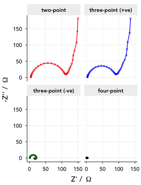
I have to keep the force leads connected to the positive and negative electrodes of the cell of course, but if I move around the sense leads I can measure different contributions from the different components of the cell:
two-point measurement – I can keep the sense leads connected to the positive and negative electrodes along with the force leads, and leave the reference electrodes disconnected. This way, I’ll simply measure the impedance response of the entire cell.
three-point measurements – I can measure the potential between one of the cell electrodes and one of the references – if I measure between WE and RE1, I’ll just measure the impedance of the positive electrode. Alternatively, I can measure between CE and RE2, and measure the impedance of the lithium metal negative electrode.
four point measurement – or, I can go really crazy, and measure between RE1 and RE2. Then, the equivalent circuit is just a resistor, corresponding to the ionic resistance of the electrolyte between the two references.
Below are the Nyquist plots for these different combinations. Can you see how the different parts of the equivalent circuit combine?
Note: lithium metal is, unfortunately, not a very stable or well-behaved electrode, and shows some difficult-to-model behaviour towards lower frequencies.
Get involved
Fitting With Real Data
1366 words (7 min) Matthew Lacey 28 Mar 2023
Info
This content has been transferred from lacey.se and is not updated for this site yet.
I know from personal experience that knowing the basics well enough to interpret a very simple and well-defined experiment is one thing – but actually taking that knowledge and trying to make sense of the response of a complex ‘real’ system is another.
As equivalent circuits become more complicated, they become harder to fit correctly. Impedance software uses non-linear least squares regression to fit the data to the models, and they need reasonable values to start with to converge on a solution. The more complicated the model gets, the more likely the software is to fail in its attempt to fit the data – or it returns a fit which looks ok on the plot but has huge errors for some of the terms.
It’s this aspect of practical EIS which I think makes it hard to learn, and I don’t think there’s a lot of help out there for users who don’t have the luxury of being able to consult a local expert.
On the previous page, on three- and four-electrode measurements, I showed some real data from a Li-ion test battery just after assembly, and a rather complicated suggested equivalent circuit for it. You might have also recognised that the Nyquist plot for the positive electrode (taken from a 3-electrode measurement) was the same as I showed on the main page of this guide (shown again on the right) – and maybe you’re wondering where the equivalent circuit came from.
Well, the equivalent circuit I’ve chosen is somewhat empirical – and I’m not going to guarantee that it’s the most appropriate possible circuit – but I figured it makes a convenient example to show you how you can approach fitting a more complex dataset. On this page I’ll detail the process I used to analyse the data by eye and build up the model.
Equivalent circuit fitting in ZView
The screenshots I present here are from ZView, which can be downloaded from the software manufacturer, although the latest versions will only run in ‘demonstration mode’ – which is basically unusable – unless you have an expensive licence. Older versions (e.g. 3.2b) are ok, and Google may help you find it…
Ok, to the data. Let’s look at the spectrum above again, and pretend the fit line isn’t there. What are the obvious features? Well, there’s the slightly depressed semicircle at high frequency, and then the behaviour is pseudocapacitive at lower frequencies (lowest frequency is 100 mHz, incidentally).
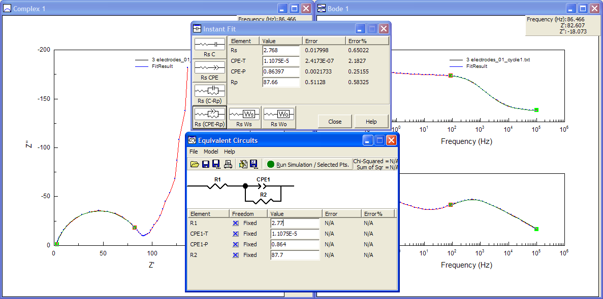
Essentially, the strategy I use is quite simple: fit the obvious stuff first, and then build up the rest of the model around that. Have a look at the following screenshot (you can click on it to enlarge it):
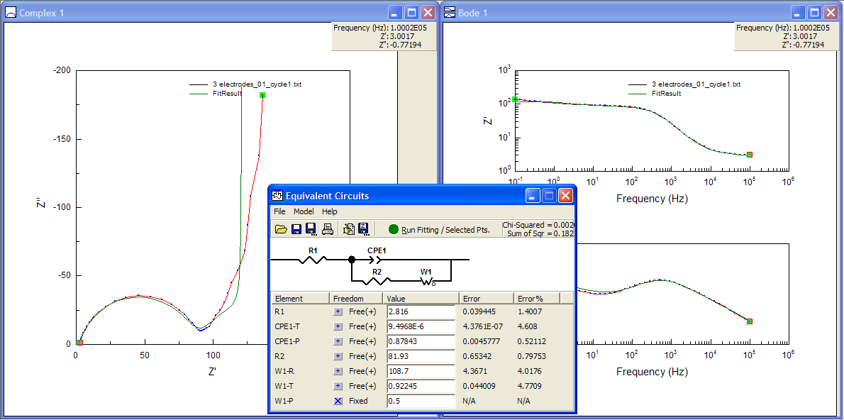
ZView lets you use sliders to fit only a part of the data if you want, and this is invaluable. Also very useful is ZView’s “Instant Fit” tool, which will fit the selected data only to any of six very simple equivalent circuits, without needing any starting values from the user. So a good place to start here, especially if you have no idea what values might be appropriate, is to fit the semicircle with the Rs (CPE-Rp) circuit (bottom-right in the Instant Fit window). As you can see, the fit is pretty good, with small errors, so I’ll take the numbers from the Instant Fit and start building up my own model in “Equivalent Circuits”.
Now to fit the low-frequency tail. I could try to fit it with a constant phase element, but the phase is obviously changing, so it’s probably not appropriate. I can try to fit it anyway just to show that it doesn’t fit well, even though the errors come out to be rather small:
The advice I often give to people who ask me about EIS measurements is that it helps to know what the spectrum should look like, although that isn’t always possible. At this point I should probably make a guess based on what I’m actually measuring. Since the electrode is for the most part a Li-ion battery positive electrode, there’s Li ions in the material which are probably moving around in response to my applied potential. So I can try to put a finite space Warburg (or “open” Warburg, in ZView language) to model that finite diffusion behaviour, instead of that CPE I tried earlier.
Well, it’s not really much better, though it makes a bit more sense… and it does fit that very first bit of the Nyquist plot after the semi-circle a bit better (the very short 45° part where Z’ ~ 90 Ω), so maybe I’m onto something.
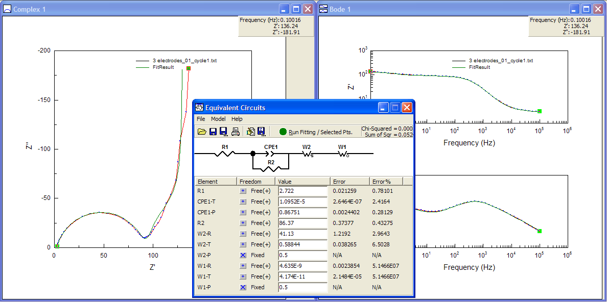
I also know that the electrode is porous, and that porosity can be represented by a finite length Warburg (or “short” Warburg, in ZView terms). So I can try to include this in the model, also in series with the FSW and the resistor R2. I fixed terms initially so that the software only guessed values for the -R (resistance) and -T (time constant) terms for the new FLW element (using 1 for each of the terms as a starting point), and then re-ran the fitting with other values freed up, keeping the phase of the Warburgs at 45° (P = 0.5).
So, now the fit is fairly decent – although the errors of 12% for the FSW element give me a little cause for concern. I could un-fix the phase angles as well – and I did, and the fit to the Nyquist plot looked better – but it caused some of the errors associated with the elements to hit more than 500%! In that case, you really can’t be sure the model is a good one.
Perhaps I can try something else. What if I try again with the Warburg elements in series with the CPE instead of in parallel with it?
Well, the fit in the Nyquist plot looks ok, similar to the last one, maybe except for that first bit of the tail… oh, wait. The values for the FSW (W1-T and W1-R) have become absurdly small and the errors are 50 million percent! That’s a telltale sign of having screwed up.
Wrap-up
Well, I concede I probably haven’t reached anything conclusive here, but if you’re new to EIS you now hopefully have at least a bit of an idea of how you can approach an equivalent circuit fitting, and some appreciation for some of the difficulties.
It’s an anticlimax, I suppose, but I do have a reason. When I was a lab teacher for EIS at the Southampton Electrochemistry Summer School, we ran a few very well-designed experiments which we knew would give easy-to-understand results; the most in-depth experiment was an analysis of the ferricyanide redox couple at a mirror-smooth glassy carbon electrode, where you get a very lovely Randles circuit response and it’s dead easy to fit and extract a load of meaningful parameters from. This is great for learning about the technique, but of course the delegates – mostly not academics – ultimately wanted to know how to apply it practically to their own work. We often got questions about predicting or analysing impedance spectra of much more complex systems like these, and we weren’t always able to give a clear answer.
The truth is that real-world EIS is more like this example here, in my experience. The more you want to learn the more you have to think about the design of the experiment, sometimes you have to take an educated guess at an appropriate equivalent circuit, and even then it can be difficult to be sure. Hence this example – it was genuinely my first attempt at fitting this data, so this was my real thought process.
Perhaps I’ve ended this example pessimistically. I don’t mean to – EIS is still a very useful technique. It’s fast, you get a lot of information that few other techniques can give you as easily – but sometimes you’ve got to be realistic about how much quantitative analysis you can do with it, and careful that when you do that analysis, the model and numbers make sense.
Get involved
Recommended Reading
623 words (3 min) Matthew Lacey 28 Mar 2023
Info
This content has been transferred from lacey.se and is not updated for this site yet.
The following are a selection of papers which I think are especially useful for further reading on specific topics. For the most part they are quite focused, and elaborate on some of the topics discussed in the pages on this website. The list is by no means exhaustive, and if you have any suggested papers which you think could find a place in this list, please feel free to suggest them to me either by email or in the comments below.
R. de Levie, “On porous electrodes in electrolyte solutions” - key fundamental work describing the original transmission line model for porous electrodes, diffusion within pores and charge transfer reactions within porous electrodes. (with thanks to Jeremy Meyers for the suggestion)
If you’ve studied all of the previous pages in this series, why not put your new-found skills to the test with a little exercise?
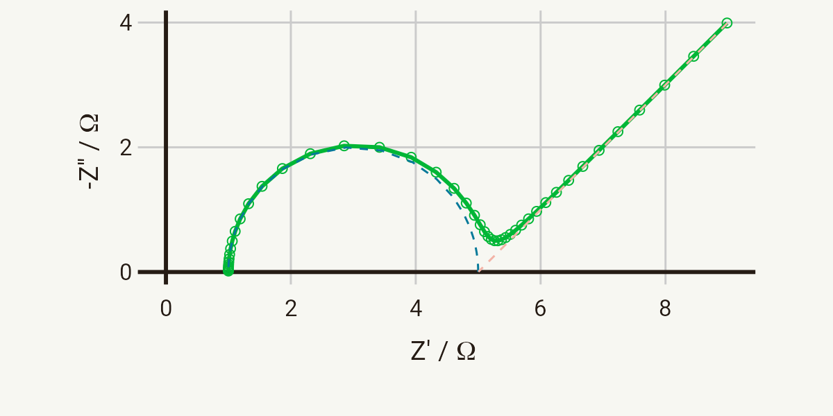
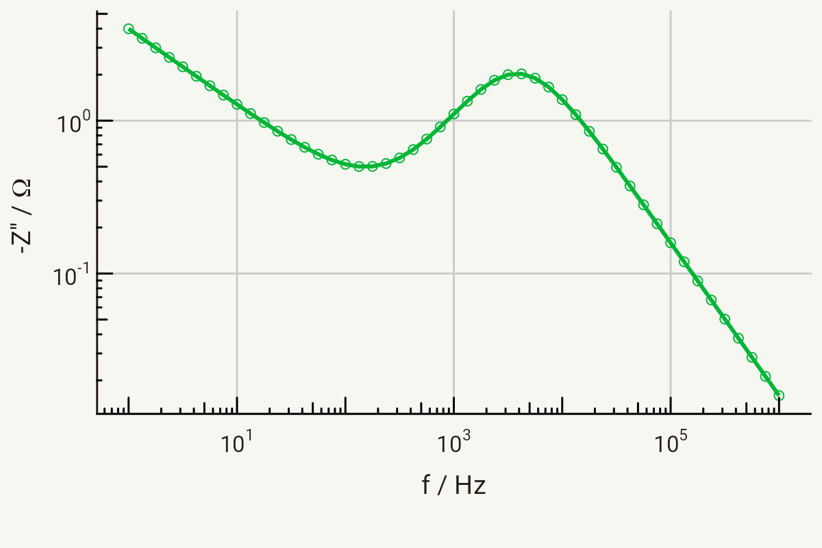
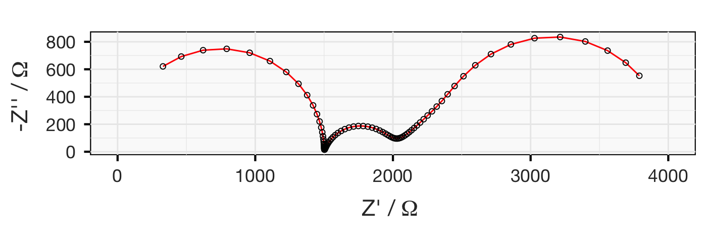
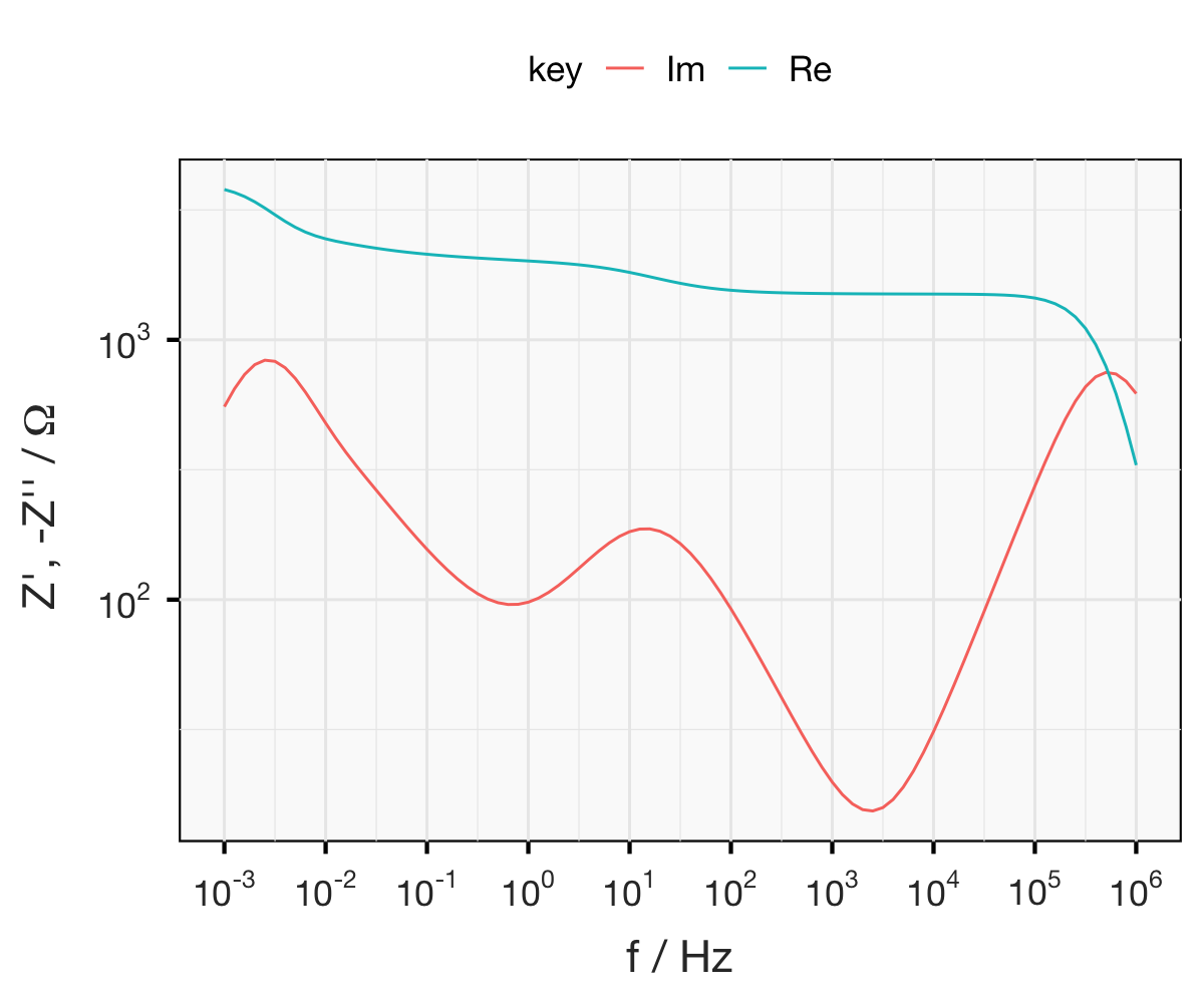
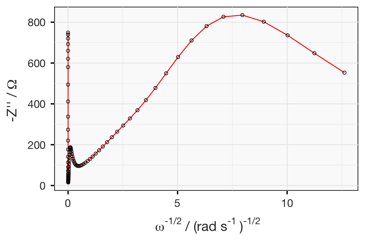
Below are three plots of simulated impedance data. The data is representative of a symmetrical electrochemical cell, comprising a thin lithium-conducting polymer electrolyte with relatively poor ionic conductivity, sandwiched between two lithium metal electrodes. (Hint: this sort of system is discussed here and here.)
Exercise: from the plots below, can you propose an equivalent circuit? Once you have come up with a circuit model, can you calculate all the relevant parameters… by hand?
This is a tricky exercise. See how far you get - and if you’re done or can go no further, why not try your hand at fitting the “raw” data? You can download the data here.
A little about this exercise
This exercise is a variant of one I used in teaching on a number of occasions. There are several aims here, which I believe test some of the most important skills for building real competence in the technique:
To understand how to propose a reasonable equivalent circuit, based on what one knows about the system under study and what features can be seen in the data
To understand how impedance data can be plotted and what information it provides
To be able to calculate parameters by hand, at least as a way to give initial guesses to the fitting software, so it can refine the fit for more complex models
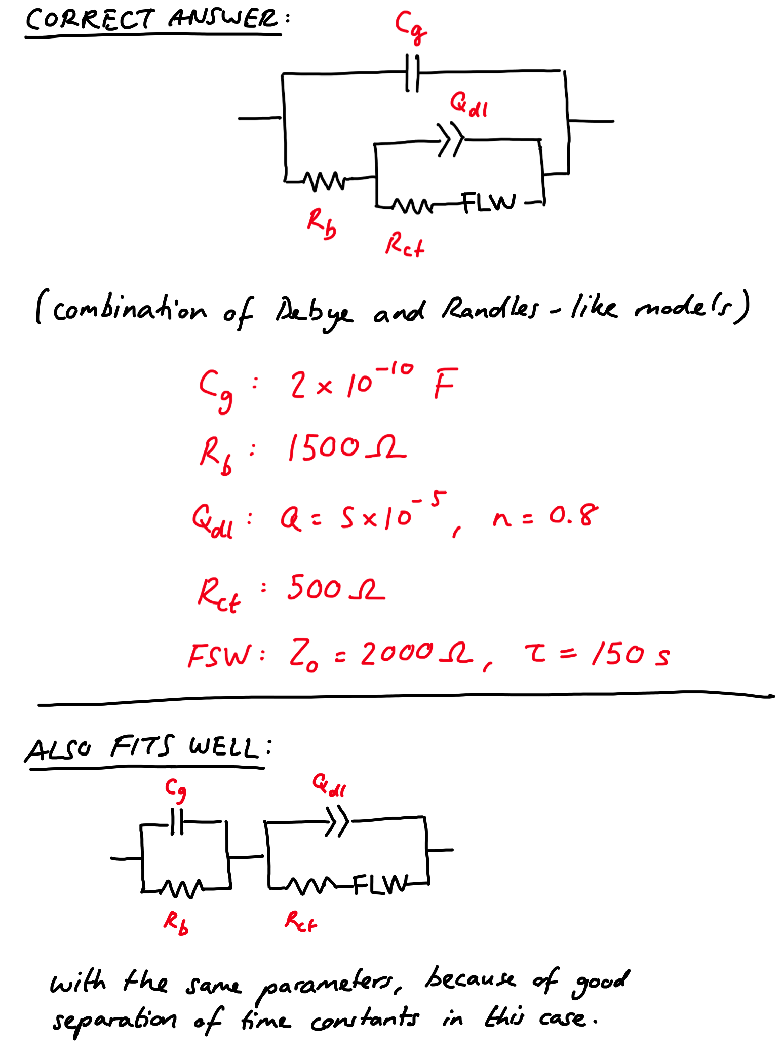
Want to check your answers? You can check how you did against the real circuit and parameters by following this link. Don’t cheat!


